文書の過去の版を表示しています。
総合演習
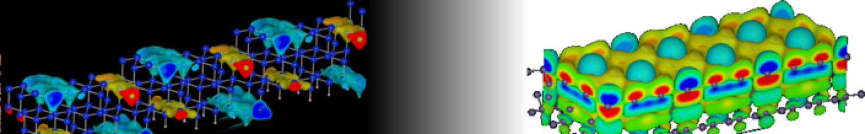
グラフェンを例に、より詳しい計算の演習を行おう。
単位格子の設定
# ----------------------
# Constant parameters
# ----------------------

a0 = 2.461 # Lattice constant of Graphene


# ----------------------
# Setting up unit cell
# ----------------------
from math import sqrt
root3 = sqrt(3.0)
ax = a0*sqrt(3.0)/2.0
ay = a0/2.0
az = a0*8.0 # Height of 3D unit cell

c1 = ( ax, ay, 0.0)
c2 = (-ax, ay, 0.0)
c3 = (0.0, 0.0, az)

unit_cell = [c1, c2, c3] # Unit cell
原子の情報の設定
# -------------------------
# Elements and positions of
# atoms in the unit cell
# -------------------------
from ase import Atom
atom1 = Atom('C', (1.0/3.0, 2.0/3.0, 0.5))
atom2 = Atom('C', (2.0/3.0, 1.0/3.0, 0.5))

list_of_atoms = [atom1, atom2]
計算パラメーターの設定
<code python> # ————————- # Calculational conditions # ————————- kwargs = {} kwargs['nbands'] = 8 # Number of Valence electrons kwargs['kpts'] = (2, 2, 1) # k-point sampling in the 1st BZ kwargs['pw'] = 150 # Energy cutoff for wave functions kwargs['dw'] = 150 # Energy cutoff for charge density </python>
計算の実行
<code python> # ————————— # Common part of calculations # ————————— from ase import Atoms box1 = Atoms(list_of_atoms, pbc = True) box1.set_cell(unit_cell, scale_atoms = True) from ase.calculators.jacapo import Jacapo solver1 = Jacapo(**kwargs) box1.set_calculator(solver1) solver1.calculate() </python>
結果の出力
<code python> # —————— # Output on screen # —————— print box1.get_total_energy() </python>